LINEAR TIME INVARIANT –CONTINUOUS TIME SYSTEMS
System:
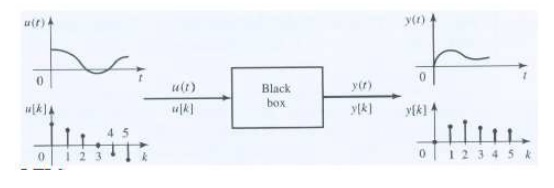
A system is an operation that transforms input signal x into output signal y.
LTI Systems
Time Invariant
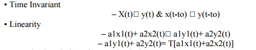
Meet the description of many physical systems
They can be modeled systematically
– Non-LTI systems typically have no general mathematical procedure to obtain solution
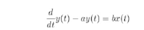
Differential equation:
This is a linear first order differential equation with constant coefficients (assuming a and b are constants)
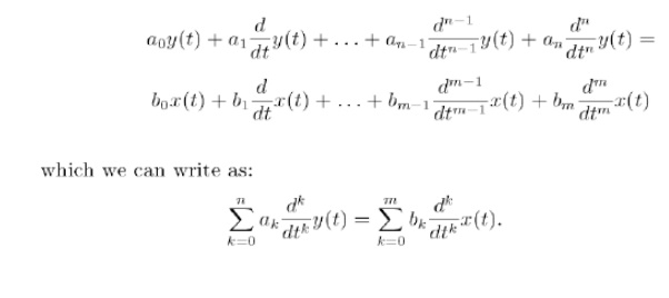
The general nth order linear DE with constant equations is
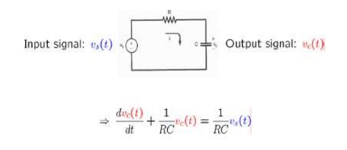
Linear constant-coefficient differential equations In RC circuit
- To introduce some of the important ideas concerning systems specified by linear constant-coefficient differential equations ,let us consider a first-order differential equations:
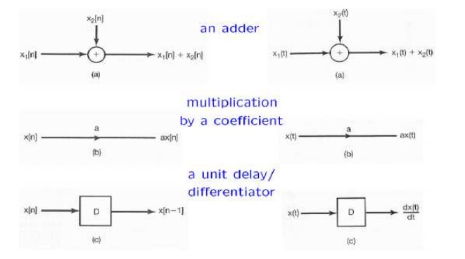
Block diagram representations
Block diagram representations of first-order systems described by differential and difference equations
Impulse Response
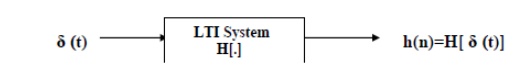
This impulse response signal can be used to infer properties about the system’s structure (LHS of difference equation or unforced solution). The system impulse response, h(t) completely characterizes a linear, time invariant system
Properties of System Impulse Response
Stable
A system is stable if the impulse response is absolutely summable
Causal
A system is causal if h(t)=0 when t<0
Finite/infinite impulse response
The system has a finite impulse response and hence no dynamics in y(t) if there exists T>0, such that: h(t)=0 when t>T
Linear
ad(t)=ah(t)
Time invariant d(t-T) = h(t-T)
Convolution Integral
An approach (available tool or operation) to describe the input-output relationship for LTI Systems
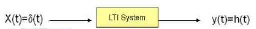
In a LTI system
d(t) # h(t)
Remember h(t) is T[d(t)]
Unit impulse function - the impulse response
It is possible to use h(t) to solve for any input -output relationship
Any input can be expressed using the unit impulse function
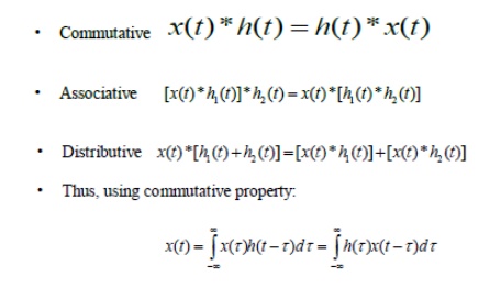
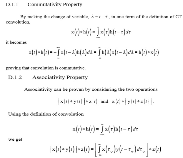
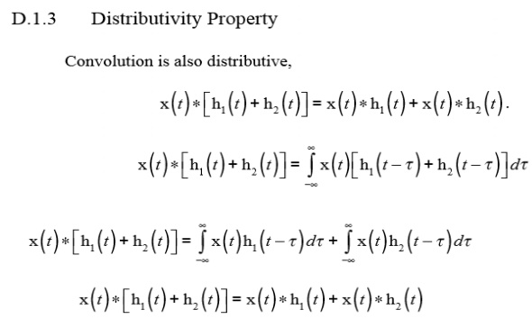
Convolution Integral - Properties
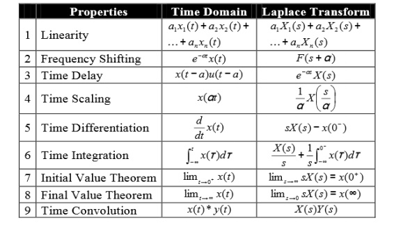
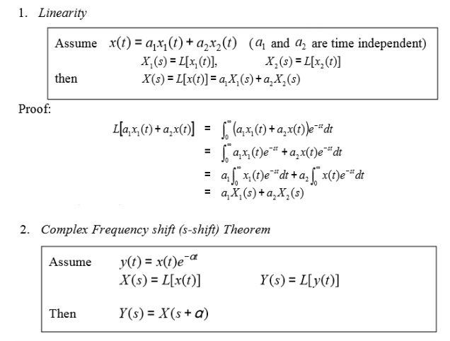
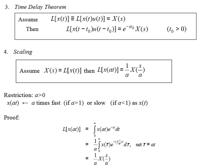
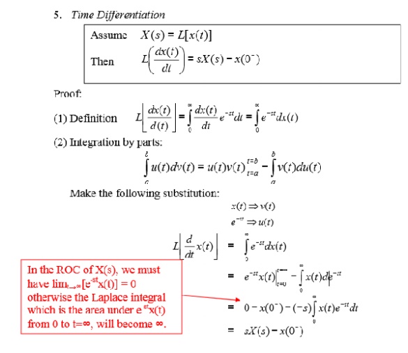
Properties of Laplace Transform:
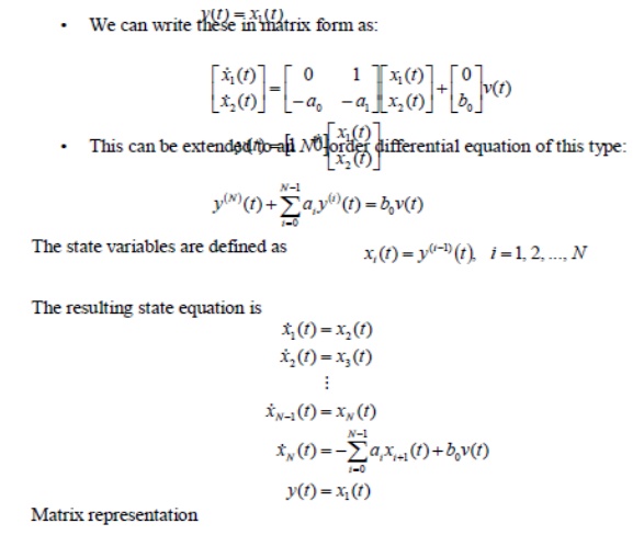
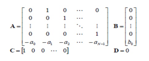
State variables and Matrix representation
• State variables represent a way to describe ALL l inear systems in terms of a common set of equations involving matrix algebra.
• Many familiar properties, such as stability, can be derived from this common representation. It forms the basis for the theoretical analysis of linear systems.
• State variables are used extensively in a wide range of engineering problems, particularly mechanical engineering, and are the foundation of control theory.
• The state variables often represent internal elements of the system such as voltages across capacitors and currents across inductors.
• They account for observable elements of the circu it, such as voltages, and also account for the initial conditions of the circuit, such as energy stored in capacitors. This is critical to computing the overall response of the system.
• Matrix transformations can be used to convert fro m one state variable representation to the other, so the initial choice of variables is not critical.
• Software tools such as MATLAB can be used to perform the matrix manipulations required.
• Let us define the state of the system by an N-element column vector, x(t):
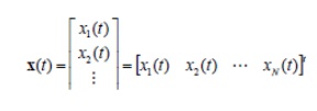
Note that in this development, v(t) will be the input, y(t) will be the output, and x(t) is used for the state variables.
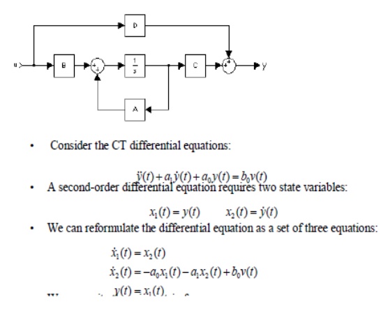
• Any system can be modeled by the following state equations:
• This system model can handle single input/single output systems, or multiple inputs and outputs.
• The equations above can be implemented using the signal flow graph shown to the below