LINEAR TIME INVARIANT DISCRETE TIME SYSTEMS
1. Introduction
A discrete-time system is anything that takes a discrete-time signal as input and generates a discrete-time signal as output.1 The concept of a system is very general. It may be used to model the response of an audio equalizer . In electrical engineering, continuous-time signals are usually processed by electrical circuits described by differential equations.
For example, any circuit of resistors, capacitors and inductors can be analyzed using mesh analysis to yield a system of differential equations. The voltages and currents in the circuit may then be computed by solving the equations. The processing of discrete-time signals is performed by discrete-time systems. Similar to the continuous-time case, we may represent a discrete-time system either by a set of difference equations or by a block diagram of its implementation.
For example, consider the following difference equation. y(n) = y(n-1)+x(n)+x(n-1)+x(n-2) This equation represents a discrete-time system. It operates on the input signal x(n)x(n) to produce the output signal y(n).
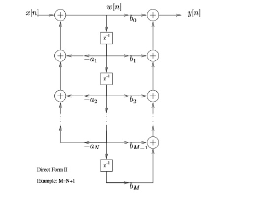
2. BLOCK DIAGRAM REPRESENTATION
Block diagram representation of
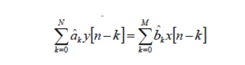
LTI systems with rational system function can be represented as constant-coefficient difference equation
• The implementation of difference equations requires delayed values of the
– input
– output
– intermediate results
• The requirement of delayed elements implies need for storage
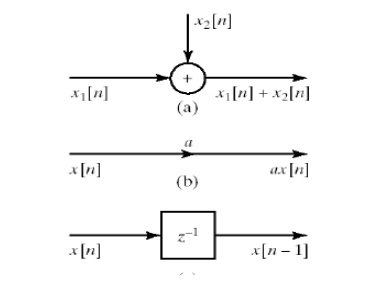
We also need means of
– addition
– multiplication
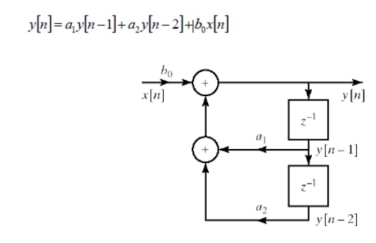
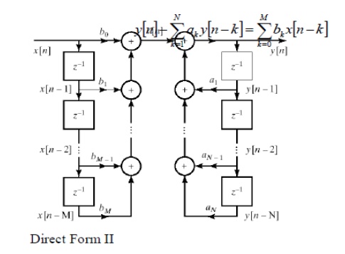
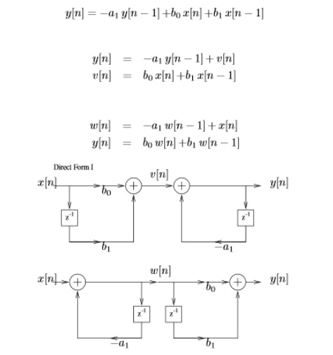
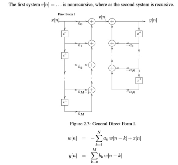
Direct Form I
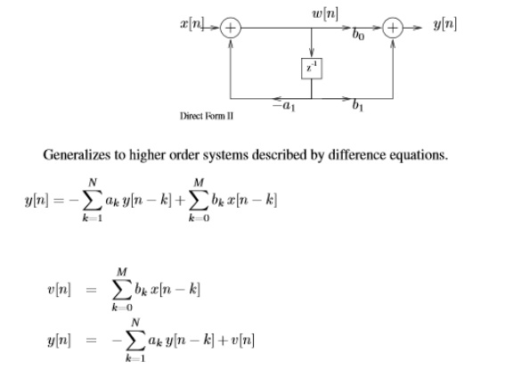
General form of difference equation
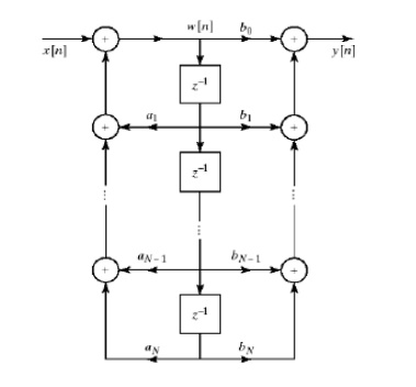
Alternative equivalent form
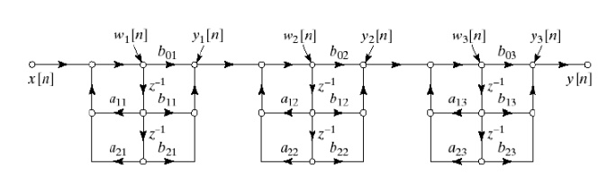
• Cascade form
General form for cascade implementation
Parallel form
Represent system function using partial fraction expansion
3. CONVOLUTIO N SUM
The convolution sum provides a concise, mathematical way to express the output of an LTI system based on an arbitrary discrete-time input signal and the system's response. The convolution sum is expressed as
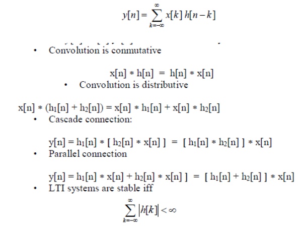
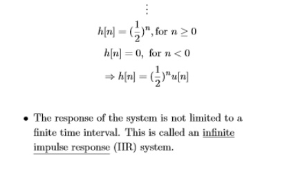
LTI systems are causal if
h[n] = 0 n < 0
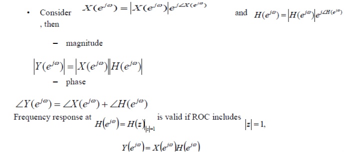
4. LTI System analysis using DTFT
LTI SYSTEMS ANALYSIS USING DTFT
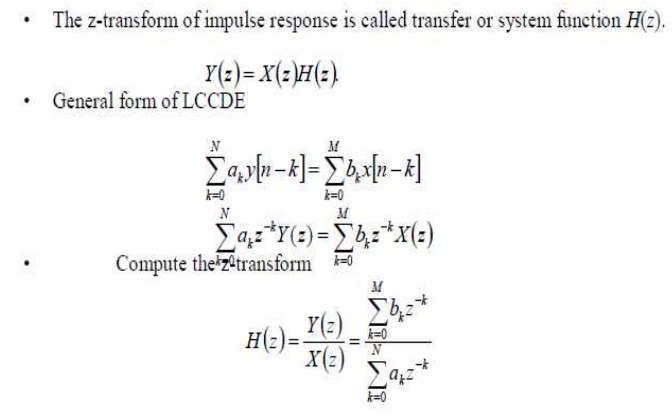
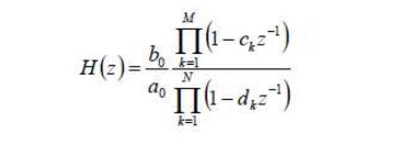
5. LTI SYSTEM ANALYSIS USING Z-TRANSFORM
The z-transform of impulse response is called transfer or system function H(z).
Y(z)=X(z)H(z)
General form of LCCDE
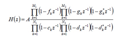
System unction: Pole/zero Factorization
Stability requirement can be verified
Choice of ROC determines causality.
Location of zero and poles determines the frequency response and phase
Sample Problems:
1. Consider the system described by the difference equation.
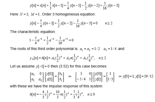
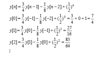
2. Given y[-1]=1 and y[-2]=0. Compute recursively a few terms of the following 2nd order DE:
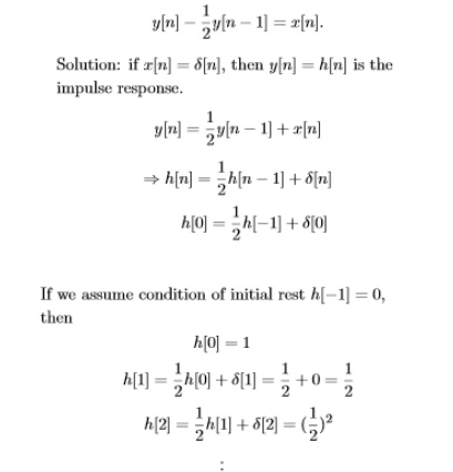
3. Compute the impulse response of the system described by,
4. Obtain the structures realization of LTI system
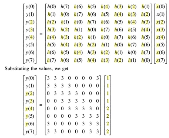
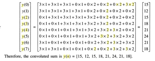
5. Find the convolution of x(n)=[1,1,1,1,2,2,2,2] with h(n)=[3,3,0,0,0,0,3,3] by using matrix method.
Solution: By using matrix method, N=8